Real World Example: Eos Well
This case study demonstrates the iterative process of geomechanical analysis using the Northern Lights dataset (courtesy of Equinor). We’ll explore how different modeling assumptions affect our results and show the importance of calibrating models with observed data.
Downloading the Data
Some extra packages are required to download using python, else we can use Azure Storage explorer to get the data using the shared access signature URI.
pip install azure-storage-blob tqdm
Now we can use the following python script to download the data to be used in this example.
from azure.storage.blob import ContainerClient
import os
from tqdm import tqdm

# use the shared access signature URI from EquiNor data sharing website after signing in.
# To create this token, go to https://data.equinor.com, and log in (either as employee or as b2c) (ensure pop-ups are allowed).
# You can create your account at this stage using your mail ID.
# Then browse to the dataset in question, in this case Northern Lights (https://data.equinor.com/dataset/NorthernLights).
# The token ("shared access signature URI") will be found at the bottom of the page, in the "Data links" section.
# The token's validity is of limited time (a month or so), you can get a new token by following the steps above once the token expires.

# Initialize the ContainerClient
container_client = ContainerClient.from_container_url("your/shared/access/signature/uri/here")

# List of files to download
files_to_download = [
   "31_5-7 Eos/06.Wireline_Log_Data/WL_RAW_AAC-ARLL-CAL-DEN-GR-NEU_RUN6_EWL_2.DLIS",
   "31_5-7 Eos/02.Drilling_and_Completion/CORING_2020-01-14_REPORT_1.PDF",
   "31_5-7 Eos/03.Directional_Surveys/WELLPATH_COMPUTED_1.ASC",
   "31_5-7 Eos/03.Directional_Surveys/WELLPATH_ORIGINAL_SURVEY_POINTS_1.ASC",
   "31_5-7 Eos/11.Core_Data/CORE_CONV_2020-05-25_REPORT_1.PDF",
   "31_5-7 Eos/12.Geology_Data_and_Evaluations/31_5-7_Formation_Tops_FWR_Sept2020.xlsx"
]

# Specify output directory with a separate variable
output_path = "."  # Relative to where the script is run from

# Create output directory if it doesn't exist
if not os.path.exists(output_path):
   os.makedirs(output_path)
   print(f"\nCreated output directory: {output_path}")

# Download each selected file
for blob_path in files_to_download:
   # Extract just the filename for local saving
   local_filename = os.path.join(output_path, os.path.basename(blob_path))

   # Get blob client and properties
   blob_client = container_client.get_blob_client(blob_path)
   properties = blob_client.get_blob_properties()
   file_size = properties.size

   print(f"\nDownloading {os.path.basename(blob_path)} ({file_size/1024/1024:.2f} MB)...")

   # Download with progress bar
   with open(local_filename, "wb") as download_file:
      download_stream = blob_client.download_blob()

      # Using tqdm for progress reporting
      progress_bar = tqdm(total=file_size, unit='B', unit_scale=True)

      # Download in chunks to show progress
      chunk_size = 1024 * 1024  # 1MB chunks
      for chunk in download_stream.chunks():
            download_file.write(chunk)
            progress_bar.update(len(chunk))

      progress_bar.close()

   print(f"Successfully downloaded {os.path.basename(blob_path)}")

print("\nAll files downloaded successfully!")
The downloaded data will be used in the following example, with some files created based on the information downloaded (by changing the file types and format as required) Some of the data required for this example has strict format requirements, we provide example versions with current formatting in the following repository: https://github.com/GeoArkadeep/supporting-data-for-EOS-Northern-Lights
# Load support data

import pandas as pd

survey = pd.read_csv('https://raw.githubusercontent.com/GeoArkadeep/supporting-data-for-EOS-Northern-Lights/main/Deviation.csv')
print(survey)
formations = pd.read_csv('https://raw.githubusercontent.com/GeoArkadeep/supporting-data-for-EOS-Northern-Lights/main/NorthernLights-31_5-7.csv')
print(formations.head())
print(list(formations))

"""
   Top TVD  Number                  Formation Name  ...  DXP_NCT  DXP_exp  DXP_ML
0      488       1  URU(Upperregionalunconformity)  ...      NaN      NaN     NaN
1      772       2                           Skade  ...      NaN      NaN     NaN
2     1144       3              HordalandGreenClay  ...      NaN      NaN     NaN
3     1442       4                          Balder  ...      NaN      NaN     NaN
4     1530       5                            Sele  ...      NaN      NaN     NaN

[5 rows x 24 columns]
['Top TVD', 'Number', 'Formation Name', 'GR Cut', 'Struc.Top', 'Struc.Bottom', 'CentroidRatio',
'OWC', 'GOC', 'Coeff.Vol.Therm.Exp.', 'SHMax Azim.', 'SVDip', 'SVDipAzim', 'Tectonic Factor',
'InterpretedSH/Sh', 'Biot', 'Dt_NCT', 'Dt_ML', 'Res_NCT', 'Res_Exp', 'Res_ML', 'DXP_NCT', 'DXP_exp', 'DXP_ML']
"""
# The formations data, if provided, must contain 24 columns in this exact order.
# If values are unavailable or we wish to use the defaults/constant values, it is fine to leave them blank

ucs = pd.read_csv('https://raw.githubusercontent.com/GeoArkadeep/supporting-data-for-EOS-Northern-Lights/main/UCSdata.csv')
print(ucs.head())
"""
   2643.08  35
0  2644.02  34
1  2645.02  35
2  2646.25  31
3  2647.50  37
4  2648.55  34
"""
# The UCS data if provided, must be in MPa, with the depths in metres, TVD.

imagelog = pd.read_csv('https://raw.githubusercontent.com/GeoArkadeep/supporting-data-for-EOS-Northern-Lights/main/31_5-7_Image.csv')
#Image log is available and features are visible, so we will use them here.
Initial Setup
First, let’s import the required packages:
import stresslog as lst
from welly import Well
Loading Well Data
Here’s how we load our well data:
alias = {
   "sonic": ["none", "DTC", "DT24", "DTCO", "DT", "AC", "AAC", "DTHM"],
   "ssonic": ["none", "DTSM","DTSH_FINAL"],
   "gr": ["none", "GR", "GRD", "CGR", "GRR", "GRCFM","GR_EDTC"],
   "resdeep": ["none", "HDRS", "LLD", "M2RX", "MLR4C", "RD", "RT90", "RLA1", "RDEP", "RLLD", "RILD", "ILD", "RT_HRLT", "RACELM"],
   "resshal": ["none", "LLS", "HMRS", "M2R1", "RS", "RFOC", "ILM", "RSFL", "RMED", "RACEHM", "RXO_HRLT"],
   "density": ["none", "ZDEN", "RHOB", "RHOZ", "RHO", "DEN", "RHO8", "BDCFM"],
   "neutron": ["none", "CNCF", "NPHI", "NEU", "TNPH", "NPHI_LIM"],
   "pe": ["none", "PEFLA", "PEF8", "PE"]
}

# Load well log data
vertwell = lst.get_well_from_dlis('WL_RAW_AAC-ARLL-CAL-DEN-GR-NEU_RUN6_EWL_2.DLIS', aliases=alias, step=0.147)
# we could have used aliases=None (which is the default) but that would have returned ALL the channels in the dlis creating a huge las file which slows the analysis somewhat.
# also steps less than 0.15m will be reset to 0.15m, this is a protective measure, upsampling data beyond it's natural resolution with this method creates artefacts and other issues.
Iteration 1: Vertical Well
Our first analysis assumes a vertical well:
# Set up mud KB, GL, BHT and LOT values
attrib = [50, -307, 0, 0, 0, 100, 0, 0]
xlot = [[1.43, 2582.9]]
# Create vertical well model
wellwithoutdeviation = lst.getwelldev(wella=vertwell, deva=None)
# Run initial analysis
output = lst.compute_geomech(
wellwithoutdeviation,
attrib=attrib,
rhoappg=17.33,
a=0.8,
lamb=0.00075,
forms=formations,
UCSs=ucs,
writeFile=True,
user_home="./output",
offset=91,
dip_dir=180,
dip=2,
doi=2627.5,
mwvalues=[[1.26, 0.0, 0.0, 0.0, 0.0, 0]],
plotstart=2560,
plotend=2660,
mudtemp=35,
fracgradvals=xlot,
)
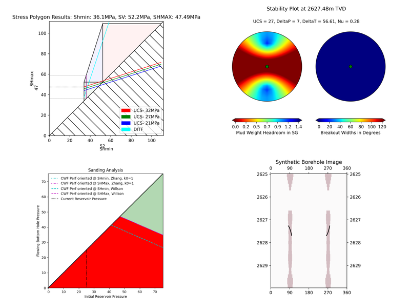
# Let's check the "PlotAll.png" in the output/Stresslog_Plots to see the zobackogram, stability plot, sanding risk plot and synthetic borehole image
# Let's also compare the "PlotBHI.png" to the actual image log of the Northern Lights Eos well
# While the inbuilt plotting tools work, the main output is the dataframe (and the las string generated from the dataframe and other info)
print(output[0])
print(list(output[0]))
"""
DEPT DTCO ... Shear_Modulus Bulk_Modulus
0 0.0000000000 NaN ... 0.0000000000 0.0000000000
1 0.1470000000 NaN ... 0.0000000000 0.0000000000
2 0.2940000000 NaN ... 0.0000000000 0.0000000000
3 0.4410000000 NaN ... 0.0000000000 0.0000000000
4 0.5880000000 NaN ... 0.0000000000 0.0000000000
... ... ... ... ... ...
19828 2914.7159999987 NaN ... 2.2818260018 6776.4871193190
19829 2914.8629999987 NaN ... 2.2820489493 6777.2354994299
19830 2915.0099999987 NaN ... 2.2822719005 6777.9839018296
19831 2915.1569999987 NaN ... 2.2824948556 6778.7323265105
19832 2915.3039999987 NaN ... 0.0000000000 0.0000000000
[19833 rows x 40 columns]
['DEPT', 'DTCO', 'DTSM', 'GR', 'NPHI', 'RLA1', 'RXO_HRLT', 'RHOZ', 'PEFLA', 'MD', 'TVDM', 'INCL', 'AZIM', 'ShaleFlag', 'RHO', 'OBG_AMOCO', 'DTCT', 'PP_GRADIENT', 'SHmin_DAINES', 'SHmin_ZOBACK', 'FracGrad', 'FracPressure', 'GEOPRESSURE', 'SHmin_PRESSURE', 'SHmax_PRESSURE', 'MUD_PRESSURE', 'OVERBURDEN_PRESSURE', 'HYDROSTATIC_PRESSURE', 'MUD_GRADIENT', 'S0_Lal', 'S0_Lal_Phi', 'UCS_horsrud', 'S0 Lal', 'phi_lal', 'phi_lang', 'Poisson_Ratio', 'ML90', 'Youngs_Modulus', 'Shear_Modulus', 'Bulk_Modulus']
"""
print(output[1][:2500])
"""
~Version ---------------------------------------------------
VERS. 2.0 : CWLS log ASCII Standard -VERSION 2.0
WRAP. NO : One line per depth step
DLM . SPACE : Column Data Section Delimiter
~Well ------------------------------------------------------
STRT.m 0.00000 :
STOP.m 2915.30400 :
STEP.m 0.14700 :
NULL. -999.25 : Null value
UWI . 31/5-7 :
WELL. 31/5-7 :
SRVC. Schlumberger :
COMP. Equinor :
FLD . Eos :
~Curve Information -----------------------------------------
DEPT .m :
DTCO .us/ft :
DTSM .us/ft :
GR .gAPI :
NPHI .m3/m3 :
RLA1 .ohm.m :
RXO_HRLT .ohm.m :
RHOZ .g/cm3 :
PEFLA . :
MD .m :
TVDM .m :
INCL . :
AZIM . :
ShaleFlag . :
RHO .gcc :
OBG_AMOCO .gcc :
DTCT . :
PP_GRADIENT .gcc :
SHmin_DAINES .gcc :
SHmin_ZOBACK .gcc :
FracGrad .gcc :
FracPressure .psi :
GEOPRESSURE .psi :
SHmin_PRESSURE .psi :
SHmax_PRESSURE .psi :
MUD_PRESSURE .psi :
OVERBURDEN_PRESSURE .psi :
HYDROSTATIC_PRESSURE.psi :
MUD_GRADIENT .gcc :
S0_Lal . :
S0_Lal_Phi . :
UCS_horsrud .mpa :
S0 Lal .mpa :
phi_lal . :
phi_lang . :
Poisson_Ratio . :
ML90 .gcc :
Youngs_Modulus . :
Shear_Modulus . :
Bulk_Modulus . :
~Params ----------------------------------------------------
SMALL_RING .in 8.0 : Caliper Calibration Small Ring
LARGE_RING .in 11.999999046325684 : Caliper Calibration Large Ring
NCT_WATER_TEMP .degC 24.444442749023438 : Calibration Tank Water Temperature
GR_JIG_REF .gAPI 160.0 : Jig minus background reference
"""
In this first run, we’ve made several key assumptions:
The well is perfectly vertical
The SHmax azimuth is 91 degrees
The stress tensor is tilted 2 degrees to the south
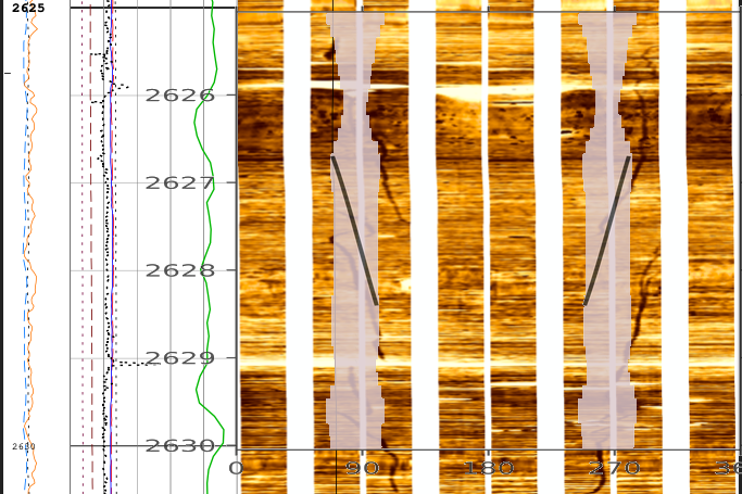
The results can be found in the ./output/Stresslog_Plots directory, where PlotAll.png shows the Zobackogram, stability plot, sanding risk plot, and synthetic borehole image. The image at ./output/Stresslog_Plots/PlotBHI.png has been overlain on the imagelog manually to compare fracture patterns.


Iteration 2: Incorporating Well Deviation
Looking at the survey data, we notice that the well isn’t perfectly vertical. At 2621.97m, there’s a slight deviation with an inclination of 0.60° at an azimuth of 40.11°. Could this slight departure from verticality explain the en-echelon fractures we observe?
# Create deviated well model
wellwithdeviation = lst.getwelldev(wella=vertwell, deva=survey)
# Run analysis with deviation but no stress tensor tilt
output = lst.compute_geomech(
    wellwithdeviation,
    attrib=attrib,
    rhoappg=17.33,
    lamb=0.00075,
    forms=formations,
    UCSs=ucs,
    writeFile=True,
    user_home="./output0",
    offset=91,
    dip_dir=180,
    dip=0,
    doi=2627.5,
    mwvalues=[[1.26, 0.0, 0.0, 0.0, 0.0, 0]],
    plotstart=2560,
    plotend=2660,
    mudtemp=35,
    fracgradvals=xlot
)
These results can be found in the ./output0/Stresslog_Plots directory, as plotBHI.png (we will be using different output directories throughout these examples, as set by the user_home parameter. In regular useage, the user_home defaults to ~/Documents, so users can find their results there by default).
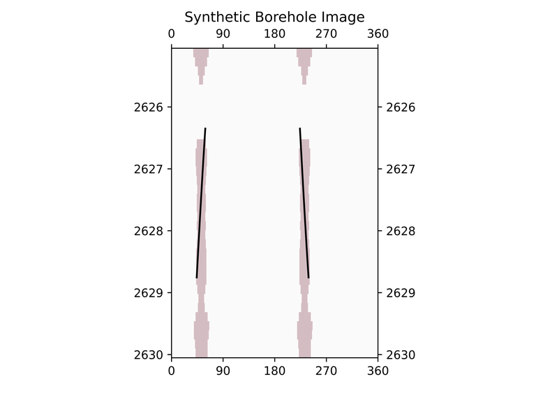
We observe that this model produces fractures with closure directions opposite to what we see in the actual image logs. This suggests our assumption about well deviation being the primary factor might be incorrect.
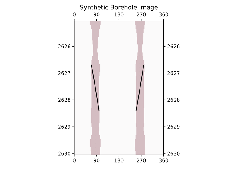
Iteration 3: Reintroducing Stress Tensor Tilt
Let’s try reintroducing the stress tensor tilt while keeping the well deviation:
output = lst.compute_geomech(
    wellwithdeviation,
    attrib=attrib,
    rhoappg=17.33,
    lamb=0.00075,
    forms=formations,
    UCSs=ucs,
    writeFile=True,
    user_home="./output1",
    offset=91,
    dip_dir=180,
    dip=2,
    doi=2627.5,
    mwvalues=[[1.26, 0.0, 0.0, 0.0, 0.0, 0]],
    plotstart=2560,
    plotend=2660,
    mudtemp=35,
    fracgradvals=xlot
)

This corrects the closure direction, but now the fracture alignment is incorrect. The results suggest we need an SHmax azimuth above 100°, closer to 120°.
Iteration 4: Using Log-Derived SHmax Azimuth
Digging deeper into the log data, we discover there’s actually a proxy for SHmax azimuth in the log itself:
# Extract SHmax azimuth from log data
y = lst.get_dlis_data('WL_RAW_AAC-ARLL-CAL-DEN-GR-NEU_RUN6_EWL_2.DLIS')
z = y[0]["FSH_AZIM_OVERALL"]
unwrapped_z = z.where(z >= 0, z + 180)

# Plot the azimuth values
from matplotlib import pyplot as plt
plt.plot(unwrapped_z)
plt.xlabel("Depth (metres)")
plt.ylabel("Fast Shear Azimuth as per log data (degrees)")
plt.savefig('SHmax_Azim.png')
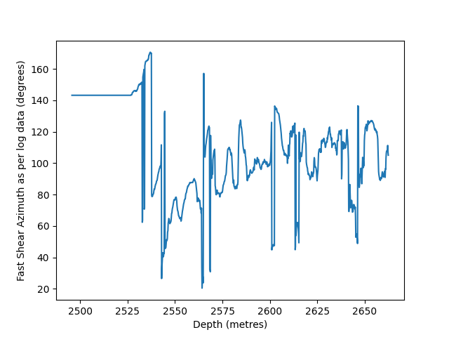
These values are significantly different from the regional database values. Nevertheless, let us try the indicated value 114°:
output = lst.compute_geomech(
    wellwithdeviation,
    attrib=attrib,
    rhoappg=17.33,
    lamb=0.00075,
    forms=formations,
    UCSs=ucs,
    writeFile=True,
    user_home="./output2",
    offset=114,
    dip_dir=180,
    dip=2,
    doi=2627.5,
    mwvalues=[[1.26, 0.0, 0.0, 0.0, 0.0, 0]],
    plotstart=2560,
    plotend=2660,
    mudtemp=35,
    fracgradvals=xlot,
    ten_fac=0
)
How about the maximum value of 124°? Clearly this is stretching things quite some, totally unrealistic I think. Here goes:
output = lst.compute_geomech(
    wellwithdeviation,
    attrib=attrib,
    rhoappg=17.33,
    lamb=0.00075,
    forms=formations,
    UCSs=ucs,
    writeFile=True,
    user_home="./output2",
    offset=124,
    dip_dir=180,
    dip=2,
    doi=2627.5,
    mwvalues=[[1.26, 0.0, 0.0, 0.0, 0.0, 0]],
    plotstart=2560,
    plotend=2660,
    mudtemp=35,
    fracgradvals=xlot,
    ten_fac=0
)
Discussion
There are some important caveats to consider:
The SHmax_Azim values in the log actually range from 90° to 125° in the interval containing the fractures.
If these varying azimuths (as seen at the log scale) were indeed effecting the fracture pattern, we would expect to see considerable variation in fracture position, which is not observed in the data.
This case study illustrates the complexity of real-world geomechanical analysis. Which model (if any) better describes reality is left upto the geological sensibility of the reader.